jMetrik 4 User Guide

Compute correlations among two or more numeric variables. Correlations use the original data, not the item scores. jMetrik will display the correlation and covaariance matrix for the selected variables.

• Click Analyze > Correlation to start the dialog.
• Select two or more variables.
• Select the Listwise deletion option to omit a case with missing data on any variable. Alternatively, choose the Pairwise deletion option to omit cases without data on one or both variables in a pair. Pairwise deletion may result in a different sample size for each pair of variables.
• If you would like to see the standard error of the correlation coefficient and a p-value for the null hypothesis that r = 0.0, select the option to Show standard error.
• By default, correlations will use an Unbiased estimator (i.e. n-1). If you would like to use a biased estimator (i.e. n), choose the Biased option.
• Click the Run button to execute the analysis.

Descriptives statistic provide various univariate summaries of each selected variable. Only numeric data will appear in the dialog’s variable list. Computations use the actual values in the data set, not the item scores.

• Click Analyze > Descriptives to start the dialog.
• Select one or more variables.
• Click the Run button.

There are many ways to conduct a differential item functioning (DIF) analysis. jMetrik provides several useful statistics including the Mantel-Haenszel chi-square procedure, commons odds ratio effect size, standardized p-dif effectsize, and ETS DIF classification levels. These statistics allow you to judge the statistical and practical significance of DIF. You must complete item scoring before you conduct a DIF analysis. See FAQ #8 for more information about the DIF analysis options and output. To conduct a DIF analysis you need a matching variable such as a sum score. If one does not exist in your data table, you must create it using the Test Scaling procedures and possibly the Ranking procedures.

• Create a matching variable – If a matching variable does not exist in your data you can create one by computing a sum score. See the instructions for Test Scaling for directions on how to create a sum score. If a matching variable exists, then use it in the next step.
• Choose thick or thin matching – Thin matching involves all levels of a sum score. To use thin matching, select a sum score variable as your matching variable in a DIF analysis. This method provides the best control over the measured trait, but it may result in sparse tables and omitted responses. Think matching preserves more of the data but gives you less control over the measured trait. For think matching group examinees into ordered groups such as deciles. Use the Deciles option of the Ranking procedure to rank examinees into ten groups. Use the new decile variable as your matching variable in the DIF analysis.
• Click Analyze > DIF: Mantel-Haenszel to start the DIF analysis dialog.
• Select the items you would like to study and move them to the top right list by clicking the first select button.
• Select the matching variable and move it to the Matching Variable field by clicking second select button.
• Select the DIF grouping variable and move it to the Group By field by clicking the last select button. An example grouping variable is gender.
• Identify the Focal and reference group codes that are in your grouping variable. For example, the code F might indicate females in your DIF group variable and the code M might represent males. The case of the focal and reference group codes must match the case of the values listed for the DIF group variable. IF you use the wrong case, the program will not recognize the values in the group variable.
• You can run the analysis at this point, but you may want to change some of the default options.
  • Binary item effect size – The default value is Common odds ratio option. This statistic ranges from 0 to positive infinity and has an expected value of unity. To use a more symmetric effect size, choose the ETS Delta option. The ETS statistic is a transformation of the common odds ratio that has values that range from about -4 to +4 and are centered about zero. Note that the polytomous item effect size is always the Standardized P-DIF statistic.
  • Show frequency tables – Select this option to display frequency tables for all levels of the matching variable. Choosing this option will greatly increase the output.
  • Score as zero – Select this option to score missing item responses as zero points. If not selected examinees missing an item response for an item will be omitted from the analysis of that item.
• If you would like to save item statistics in a new database table, click the Save button and type a name for the new table.
• Click the Run button to execute the analysis.

Frequency tables give you frequencies, cumulative frequencies, percentages, and cumulative percentages for each selected variable. Computations use the actual values in the data set, not the item scores.

• Click Analyze > Frequencies to start the dialog.
• Select one or more variables.
• Click the Run button.

Item analysis has been a part of jMetrik since its inception. It is available for variables with item scoring information. See Item Scoring in this guide if you need to complete item scoring before running an item analysis. You can conduct an item analysis with data from binary (e.g. multiple-choice) and polytomous (e.g. constructed response) test items. Item analysis provides classical item statistics and reliability estimates for your test items. In particular it provides item difficulty (i.e. pvalue, the mean item score), item discrimination (i.e. item-total correlaiton), and a distractor analysis for each item. Reliability estimates include KR-21, coefficient alpha, Guttman’s Lambda 2, Feldt-Gilmer, Feldt-Brennan, and Raju measures of internal consistency. Reliability confidence intervals and standard errors of measurement are also provided.

• Click Analyze > Item Analysis to start the dialog.
• Choose the items you would like included in the analysis. (Note: If no variables appear in the dialog, you have not provided item scoring. See Item Scoring in this guide for more information.)
• You can run the analysis with the default options, or change them to suit your needs. The available options are:
  • Compute item statistics – Select this option to include item statistics. If not selected, only reliability estimates will be computed.
  • Item deleted reliability – Choose this option to see a table with item deleted reliability estimates. The table will show reliability estimates when each item has been omitted from the analysis. This helps you choose which item to remove to improve reliability.
  • All response options – If selected, the output will show a complete distractor analysis. If not selected, only item difficulty and discrimination for the correct answer (binary item) or overall item score (polytomous item) will be computed.
  • Listwise deletion – If selected, an examinee will be omitted from the analysis if missing data on any item. This could result in large amounts of missing data and it is not recommended. If not selected, missing item responses will be scored as zero points and included in the analysis.
  • Correct for spuriousness – If selected, the item-total correlation (or distractor total correlation) will be adjusted to account for inclusion of the item score in the test score. That is, it will produce an item-remainder correlation, where the remainder is the test score without the studied item. If not selected, no adjustment will be made.
  • CSEM – Select this option to compute the conditional standard error of measurement. A table will be added to the output with this informaiton.
  • Show headers – Select this option to add a header before each item in the output.
  • Unbiased covariance – If not selected, correlations and standard deviations will use a biased estimator (n in the denominator). If selected, they will use an unbiased estimator (n-1 in the denominator).
  • Cut scores – Type one or more cut scores (on the raw score metric) separated by a white space to have jMetrik compute decision consistency indicies. A table with Huynh’s raw agreement and kappa statistics will be displayed when cut scores are provided.
  • Item-total correlation type – Select Pearson correlation to have jMetrik compute Pearson correlations (point-biserial for binary items, Pearson correlation for polytomous items). Choose Polyserial to have jMetrik compute Polyserial correlations (biserial correlaiton for binary items, polyserial correlaiton fo polytomous items).
• If you would like to save item statistics in a new database table, click the Save button and type a name for the new table.
• Click the Run button to execute the analysis.

If you are new to jMetrik, the first step to using the software is creating a new database. You only need to do this step once. Once you have created a database, open it, import data into it and begin your analysis.

• • Click Manage > New Database in the main menu to start the New Database dialog.
  • Type a name for the database. The name must not include any special characters such as !#$%^(). The underscore, _, is allowed.
  • Click the Create button and the database will be created.

Now that you have created a database, you must open it. You must also open a database each time you start jMetrik. Follow the steps for opening a database.

Each time you start jMetrik, you must open a database. You can also use these steps to switch to a different database than the one you are currently using.

• Click Manage > Open Database to start the dialog.
• Select the database from the list.
• Click the Open button.

Once the database opens, the name of the database will appear in the statusbar at the bottom of the interface. If data tables exist in your database, you will see a list of them on the left side of the jMetrik interface. Click a table to begin an analysis.

You can import an almost unlimited number of tables into a database. The only limit to the number of tables is the size of your computer’s hard drive. Once it is full, you cannot import data. You can import delimited files into jMetrik. Acceptable delimiters include commas, semicolons, colons, and tabs.

• Make sure you have an open database.
• Click Manage > Import Data to start the dialog.
• Type a name for the table in the Table Name text field.
• Click the Browse button to start a dialog that allows you to select the delimited file on your computer. This dialog also allows you to choose two important options. If your data file has variable names in the first row, select the In first row optoin. If not, then choose the None option. Making the wrong selection will produce an error while importing data. The second important option is the type of delimiter. For example, select Comma if your file is comma delimited. Select Tab if your file is tab delimited. Click the Browse button to accept your selections and return to the previous dialog.
• If you would like to add a description of you data file, type it in the Description text area. jMetrik will automatically add a description if you leave this area blank.
• Click the Import button to execute the import. You table will appear in the table list when the import is complete.

The quick-start guide provides information on using the basic item scoring tool. The steps listed below are for the Advanced Item Scoring tool. Advanced item scoring is more flexible and gives you more options for scoring items. For example, you can indicate multiple correct answers for multiple-choice items, reverse score polytomous items, or collapse categories for polytomous items.

• Select a table that contains the items you would like to score by clicking its name in the table list.
• Click Transform > Advanced Item Scoring to start the advanced item scoring dialog. This dialog contains a table with two columns.
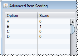• The Option column is where you enter the the response options, and the Scoring column is where you enter the score assigned to each option. Enter one option and score per row. Be sure to click on an empty cell after your last entry. jMetrik will not see your entry until you click on a new cell. The figure to the right shows and example where there are four response options A, B, C, and D with one point assigned to option B (i.e. B is the correct answer).You can also use the tool to indicate multiple correct answers. If options B and C were correct in the figure to the right, you would assign one point to each option.
• After providing the response options and scores, select the items for which you would like to apply the scoring. Click an item in the list and click the select button. Or, select each item while holding down the CTRL button on a PC and then press the select button.
• Click the Submit button to set the scoring. You can continue scoring other items. Items that already have scoring information will be in bold font in the variable list.
• After submitting the scoring information for each group of items, click the OK button to process the scoring and add it to the database. Your original data will not be changed. Item scoring is saved separately and scores are computed during an analysis. You can change the scoring information at any time.
• Scoring is also applied to polytomous items. Notice that even though numbers are provided in the data table, you must still provide scoring. This requirement allows you to reverse score polytomous items or collapse categories. The first figure 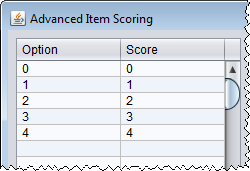 shows an example of scoring a polytomous item. Polytomous item scoring must start at 0. The second figure  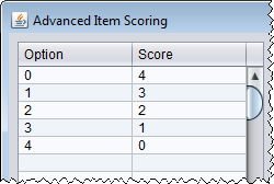shows an example of a reverse scored an item. The third image  shows an example of where options 0 and 1 have been collapsed to a score of 0, and other categories have been shifted accordingly.

Test scaling features allow you to create test scores for examinees and save the results in your data table. You can choose between a sum score, average score, Kelley regressed score, percentile rank, or normalized score. A sum score is the sum of item scores for the items selected in the dialog. Missing item responses are counted as zero points when computing a sum score. An average score is the sum score divided by the number of items completed by the examinee. As such, an average score ignores missing data and computes the score as an average score for the completed items. A Kelley regressed score is an estimate of the true score that adjusts for measurement error. If reliability equals 1, the the sum score and Kelley’s regressed score are the same. As reliability decreases, the average score for the entire group of examinees is counted toward an examinee’s Kelley score. Percentile ranks are the percentile rank of an examinee’s sum score. This method of computing percentile ranks treats data as ordered integers. Finally, a normalized score is the value from a standard normal distribution that has the same percentile rank as the sum score. Normalized scores have a mean of 0 and a standard deviatoin of 1 by default. All scores, except percentile ranks, can be linearly transformed to a new scale using the Linear Transformation panel of the dialog.

• Start the Linear Transformation dialog by clicking Transform > Test Scaling.
• In the upper part of the dialog, select all of the items that you would like to count in the score.
• In the section labeled “name,” type a name for the variable that will store the scores in the data table.
• Use the Type Combo Box to select the type of score you would like to compute.
• If no further options are needed, click the Run button to execute the analysis. A new variable will be added to the data table using the name you provided. This new variable will contain the scores for your examinees. Summary statistics and a score conversion table will be displayed in the interface.
• To apply a linear transformation such that the scores have a particular mean and standrd deviation, type numeric values in the appropriate text field in the Linear Transformation panel.
• You can specify a minimum and maximum score value by providing information in the Constraints panel.
• The Precision text field allows you to indicate the number of decimal places that you would like to impose on the scores. For example, typing 0 in the Precision text field will round scores to the nearest integer.
• Click the Run button to execute the analysis. A new variable will be added to the data table using the name you provided. This new variable will contain the scores for your examinees. Summary statistics and a score conversion table will be displayed in the interface.